How To Find Mean Median Mode Of Grouped Data

Suppose nosotros want to compare the age of students in ii schools and determine which school has more aged students. If nosotros compare on the basis of individual students, we cannot conclude annihilation. Nevertheless, if for the given information, we get a representative value that signifies the characteristics of the data, the comparison becomes like shooting fish in a barrel.

A certain value representative of the whole data and signifying its characteristics is chosen an average of the data. Three types of averages are useful for analyzing data.

They are:

(i) Mean

(ii) Median

(iii) Mode

In this commodity, we will written report three types of averages for the analysis of the information.

Mean

The hateful (or average) of observations is the sum of the values of all the observations divided by the total number of observations.

The mean of the data is given by ten = f₁ten_one + f_two10₂ + …….. + f_nx_{due north}/f1 + f2+……….. + fn

Mean Formula is given by

Mean= ∑(f_i.x_i)/∑f_i

Methods for calculating hateful

Method 1: Direct Method for calculating Mean

Step 1: For each class, detect the form mark x_i, as

             x=one/2(lower limit + upper limit)

Stride 2: Calculate f_i.x_i for each i.

Step iii: Use the formula Mean = ∑(f_i.ten_i)/∑f_i

Case: Observe the hateful of the following information.

Class Interval	0-10	10-20	20-xxx	thirty-40	twoscore-50
Frequency	12	16	6	7	9

Solution:

We may set the table given below:

Course Interval	Frequency  fi	Grade Mark xi	( fi.teni )
0-ten	12	v	lx
x-20	sixteen	15	240
20-30	6	25	150
thirty-40	vii	35	245
xl-50	9	45	405
	∑fi=50		∑fi.xi=1100

Mean=∑(f_i.ten_i)/∑f_i = 1100/50 = 22

Method 2: Assumed – Mean Method For computing Mean

For computing the mean in such cases we proceed as under.

Pace 1: For each class interval, summate the class marking x by using the formula: x_i =1/2 (lower limit + upper limit).

Step 2: Choose a suitable value of mean and denote it by A. ten in the middle as the assumed mean and announce information technology by A.

Footstep 3: Summate the deviations d_i =(x,-A) for each i.

Step 4: Calculate the product (f_i x d_i) for each i.

Step 5: Detect due north = ∑f_i

Step 6: Calculate the mean, x, by using the formula: X = A+ ∑f_id_i/n

Example: Using the assumed-hateful method, notice the mean of the following information:

Class Interval	0-10	ten-20	20-thirty	thirty-40	forty-50
Frequency	7	viii	12	13	10

Solution:

Let A=25 be the assumed hateful. And then we accept,

Grade Interval	Frequency fi	Mid value xi	Deviation di=(xi-25)	(fixdi)
0-x	seven	five	-20	-140
ten-20	8	15	-10	-80
20-thirty	12	25=A	0	0
30-xl	13	35	x	130
40-50	10	45	20	200
	∑fi=50			∑(fixdi)=100

Hateful = 10 = A+ ∑f_id_i/n = (25+110/50)=27.2

Method 3: Step-Deviation method for computing Mean

When the values of x, and f are large, the calculation of the mean by the higher up methods becomes ho-hum. In such cases, nosotros use the pace-deviation method, given beneath.

Step 1: For each form interval, calculate the class marker x,, where X = 1/2 (lower limit + upper limit).

Step 2: Choose a suitable value of x, in the centre of the x, column as the assumed mean and denote it past A.

Step three: Calculate h = [(upper limit)-(lower limit)], which is the same for all the classes.

Stride 4: Calculate u_i = (10_i -A) /h for each course.

Step five: Calculate fu for each class and hence find ∑(f_i 10 u_i).

Step 6: Calculate the hateful by using the formula: ten = A + {h x ∑(f_i x u_i)/ ∑f_i}

Example: Detect the hateful of the following frequency distribution:

Class	50-lxx	70-xc	90-110	110-130	130-150	150-170
Frequency	18	12	xiii	27	8	22

Solution:

Nosotros prepare the given tabular array beneath,

Course	Frequency fi	Mid Value xi	ui=(xi-A)/h =(teni-100)20	(fixui)
50-70	18	60	-2	-36
lxx-ninety	12	fourscore	-ane	-12
90-110	13	100=A	0	0
110-130	27	120	1	27
130-150	8	140	2	sixteen
150-170	22	160	iii	66
	∑fi=100			∑(fixui)=61

A=100, h=twenty, ∑f_i=100 and ∑(f_i x u_i)=61

10 = A + {h 10 ∑(f_i 10 u_i) / ∑f_i}

  =100 + {20 + 61/100} = (100+12.2) =112.2

Median

Nosotros outset arrange the given data values of the observations in ascending order. And then, if north is odd, the median is the (due north+1/two). And if north is even, then the median will be the average of the due north/2th and the (due north/ii +i)th observation.

Formula for Computing Median:

Median, Yard_e = 50 + {h ten (North/two – cf )/f}

where,

l = lower limit of median class.

h=width of median class.

f = frequency of median course,

cf = cumulative frequency of the form preceding the median class.

Due north = ∑f_i

Example: Calculate the median for the following frequency distribution.

Class Interval	0-8	viii-xvi	sixteen-24	24-32	32-40	40-48
Frequency	8	10	16	24	fifteen	7

Solution:

Nosotros may set up cumulative frequency tabular array equally given beneath,

Class	Frequency	Cumulative Frequency
0-viii	viii	viii
8-16	ten	18
xvi-24	xvi	34
24-32	24	58
32-twoscore	15	73
xl-48	vii	80
	Northward=∑fi=80

Now, North = fourscore = (Northward/two) = 40.

The cumulative frequency just greater than forty is 58 and the respective grade is 24-32.

Thus, the median grade is 24-32.

 fifty = 24, h = 8, f = 24, cf = c.f. of preceding class = 34, and (N/2) = xl.

Median, M_e = l+ h{(N/2-cf)/f}

                    = 24+8 {(40 – 34)/ 24}

                    = 26

Hence, median = 26.

Mode

It is that value of a variate that occurs most oft. More precisely, the style is that value of the variable at which the concentration of the information is maximum.

Modal Course: In a frequency distribution, the class having maximum frequency is called the modal class.

Formula for Computing Mode:

M_o = ten_k +h{(f_thou – f_thou-i)/(2f_k -f_m-one-f_m+1)}

where,

x_m = lower limit of the modal grade interval.

f_k = frequency of the modal class.

f_1000-ane= frequency of the class preceding the modal class.

f_k+one = frequency of the class succeeding the modal class.

h=width of the form interval.

Case ane: Summate the mode for the post-obit frequency distribution.

Class	0-ten	10-20	20-30	thirty-twoscore	40-50	50-sixty	60-70	lxx-80
Frequency	v	8	7	12	28	20	10	ten

Solution:

Form 40-50 has the maximum frequency, so information technology is chosen the modal grade.

x_grand= 40, h=10, f_grand=28, f_k-i=12, f_k+i=20

Mode, Chiliad_o= x_thou +h{(f_thou – f_k-ane)/(2f_k -f_grand-1-f_thou+1)}

= 40 +10{(28 – 12)/(2*28-12 – 20)}

= 46.67

Hence, mode= 46.67

Important Result-: Human relationship amongst mean, median and mode.

Style = 3(Median) – 2(Hateful)

Instance 2: Discover the mean, mode and median for the following data,

Class	0-10	ten-20	20-30	30-40	40-fifty	Total
Frequency	8	16	36	34	6	100

Solution:

We have,

Class	Mid Value ten i	Frequency fi	Cumulative Frequency	fi . ten i
0-10	five	viii	8	40
10-20	15	16	24	240
20-30	25	36	sixty	900
30-xl	35	34	94	1190
xl-50	45	6	100	270
		∑fi=100		∑fi. xi=2640

Mean = ∑(f_i.x_i)/∑f

            =2640/100

            = 26.4

Hither, Northward =100 ⇒ Due north / 2 = 50.

Cumulative frequency just greater than 50 is 60 and corresponding class is 20-xxx.

Thus, the median class is 20-30.

Hence, l = 20, h = 10, f = 36, c =  c. f. of preceding form = 24 and Due north/two=50

Median, M_e = l+ h{(Due north/two-cf)/f}

                    = 20+x{(fifty-24)/36}

Median = 27.2.

Manner = 3(median) – 2(mean) = (iii × 27.two – 2 × 26.4) = 28.8

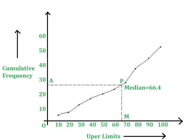
Ogives

Permit a grouped frequency distribution be given to u.s.. On a graph newspaper, we marking the upper-form limits forth the 10-centrality and the corresponding cumulative frequencies along the y-axis. On joining these points successively by line segments, nosotros get a polygon, called cumulative frequency polygon. On joining these points successively past smooth curves, we get a curve, known as ogive.

Step-by-step process for the structure of an Ogive graph

1. Showtime we marking the upper limits of course interval on the horizontal ten- axis and their corresponding cumulative frequencies on y-axis.
2. Now plot the all the corresponding points of the ordered pair given by (upper limit, cumulative frequency).
3. Bring together all the points by a free mitt.
4. The curve we become is known as ogive.

Types of Ogives

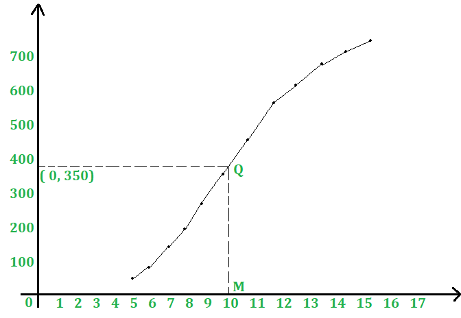
i) Less Than Ogive

On a graph paper, we mark the upper-class limits along the ten-centrality and the respective cumulative frequencies along the y-axis.

(i) On joining these points successively by line segments, we get a polygon, called cumulative frequency polygon.

(ii) On joining these points successively by smooth curves, we get a curve, known as less than ogive.

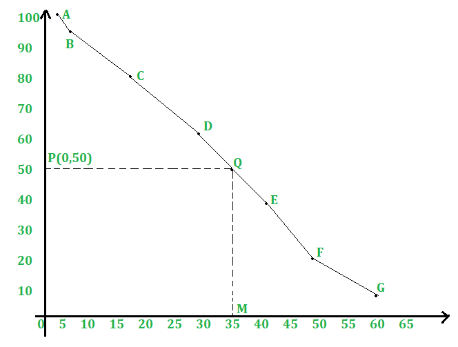
2) More than Than Ogive

On a graph paper, we mark the lower class limits along the 10-axis and the corresponding cumulative frequencies forth the y-axis.

(i) On joining these points successively by line segments, nosotros get a polygon, chosen the cumulative frequency polygon.

(ii) On joining these points successively past smooth curves, we go a curve, known as more than than ogive.

Source: https://www.geeksforgeeks.org/mean-median-and-mode-of-grouped-data/

Posted by: gillespieextesed.blogspot.com

Share this post